February 6, 2026
The "First Proof" Experiment
A group of mathematicians—including Martin Hairer, Daniel Spielman, and others—has released a provocative benchmark titled First Proof. Unlike standard AI benchmarks which rely on competition problems (IMO, AIME) or synthetic datasets, this paper presents ten private research-level questions that arose naturally in the authors' own work.
The twist? The answers are known to the authors but have never been published. They are currently hosted in an encrypted format on the project website, with the decryption key scheduled for release on February 13, 2026.
The Protocol:
The experiment tests a specific hypothesis: that current AI models can solve well-defined but deep research problems if the solution is not already in their training data. By using unpublished problems, the authors eliminate the possibility of data contamination (rote memorization).
Terence Tao noted that this structure revives the Renaissance tradition of "challenges," where mathematicians would send encrypted announcements of their discoveries (anagrams) to claim priority before revealing the proof.
Reference
-
M. Abouzaid et al.,
First Proof,
arXiv:2602.05192 (2026).
February 2, 2026
Mining the Erdős Problems
A massive collaboration led by Google DeepMind and researchers at Caltech has applied Gemini to the Erdős Problems—a database of conjectures posed by Paul Erdős.
The team focused on 700 conjectures labeled "Open." Their agent, Aletheia, utilized a hybrid approach:
- Generation: The model generated candidate proofs or counterexamples.
- Verification: A separate "verifier" routine filtered these candidates.
- Expert Review: Human mathematicians evaluated the surviving candidates.
The results were mixed but illuminating. The system successfully addressed 13 problems. However, the breakdown reveals a subtle nuance in "AI discovery":
- 5 problems were solved with seemingly novel autonomous solutions.
- 8 problems were technically "solved" by the AI, but only because the AI successfully identified that the problem had already been solved in obscure literature.
This highlights a new risk: Subconscious Plagiarism. The models occasionally reproduce arguments they have seen in their vast training corpus without attribution, presenting them as original derivations. The paper suggests that for many "open" problems, the difficulty lies not in the mathematics, but in the obscurity of the existing literature.
February 7, 2026
Rethinking R&D: The Bell Labs Architecture
Based on "How technoscientific knowledge advances: A Bell-Labs-inspired architecture" by Venkatesh Narayanamurti and Jeffrey Y. Tsao.
We often imagine innovation as a pipeline: basic science creates a discovery, applied research refines it, and development turns it into a product. This "Linear Model" is deeply embedded in how we fund and manage science. But according to Venkatesh Narayanamurti (former Dean of Harvard SEAS) and Jeffrey Tsao (Sandia National Labs), this model is fundamentally flawed—and it’s stifling modern discovery.
In their paper, they propose a different architecture for knowledge advancement, modeled after the 20th century’s most successful innovation engine: Bell Labs.
The Architecture: Bell’s "Dodecants"
Narayanamurti and Tsao argue that we must abandon the "Science vs. Technology" dichotomy. Instead, they model innovation as a 12-part grid—the Dodecants—formed by crossing Six Mechanisms of action with Two Flavors of intent.
The Six Mechanisms (The "Verbs")
The authors break down the "Scientific Method" ($\dot{S}$) and "Engineering Method" ($\dot{T}$) into three distinct steps each. These are the engines of the process:
- $\dot{S}_1$: Fact-Finding. The accumulation of new data and observations (e.g., measuring the spectral lines of hydrogen).
- $\dot{S}_2$: Explanation-Finding. Creating models or theories to make sense of facts (e.g., Bohr’s model of the atom).
- $\dot{S}_3$: Generalizing. Extending theories to cover broader classes of phenomena (e.g., Quantum Mechanics).
- $\dot{T}_1$: Function-Finding. Identifying a specific utility or need (e.g., "we need to amplify this weak signal").
- $\dot{T}_2$: Form-Finding. Designing the physical structure to achieve that function (e.g., the geometry of a transistor).
- $\dot{T}_3$: Exapting. Radical repurposing—using a technology for a completely unintended use (e.g., using a microwave radar magnetron to cook food).
The Two Flavors (The "Adverbs")
Crucially, any of the six mechanisms above can be performed with two different mindsets:
- Research Mode (R): Seeking Surprise. This is divergent thinking, aiming to disrupt current understanding or capability.
- Development Mode (D): Seeking Consolidation. This is convergent thinking, aiming to refine, stabilize, and make robust.
This creates the 12 "Dodecants." You can do "Explanation-Finding in Development Mode" (refining a known theory) or "Form-Finding in Research Mode" (trying a crazy new transistor design just to see if it switches).
The Problem: Broken Cycles
The magic of Bell Labs wasn't just having smart people; it was the fluid movement between these sectors. A physicist stuck on Explanation-Finding ($\dot{S}_2$) could walk down the hall to an engineer doing Form-Finding ($\dot{T}_2$) and realize that a manufacturing anomaly was actually a new quantum effect.
Modern R&D often breaks these cycles. "Science" grants fund only the $\dot{S}$ mechanisms, while corporate R&D funds only the $\dot{T}$ mechanisms (and usually only in "Development" mode). The Exapting ($\dot{T}_3$) mechanism—often the source of the biggest breakthroughs—is particularly starved because it fits neither pure theory nor immediate product roadmaps.
Conclusion
The decline in disruptive breakthroughs isn't due to a lack of ideas, but a rigid architecture that prevents the "Dodecants" from feeding each other. To revive the spirit of Bell Labs, we don't need more money poured into the same silos; we need to nurture the full cyclic flow between surprise and consolidation, facts and functions.
February 7, 2026
Taming Mathematical Complexity: How Software Engineering is Reshaping Pure Mathematics
Based on "Abstraction Boundaries and Spec Driven Development in Pure Mathematics" by Johan Commelin and Adam Topaz.
Modern mathematics has a scaling problem. New results are becoming increasingly intricate, often relying on deep mastery of multiple disparate subfields. Significant papers now routinely exceed one hundred pages, and the peer review process can drag on for years.
In a recent paper, Johan Commelin and Adam Topaz argue that the traditional methods of managing this complexity are hitting their limits. Their solution? Applying principles from software engineering—specifically Abstraction Boundaries and Spec Driven Development—within the rigid environment of Interactive Theorem Provers (ITPs) like Lean.
Here is how these concepts helped a distributed team of mathematicians resolve one of the most difficult challenges in modern arithmetic geometry: The Liquid Tensor Experiment.
The Problem: Inherent vs. Accidental Complexity
The authors distinguish between two types of difficulty in mathematics:
- Inherent Complexity: The raw difficulty of the ideas and the breadth of prerequisites required to understand a proof.
- Accidental Complexity: The friction caused by imperfections in communication—unwritten assumptions, ambiguous definitions, or the mental tax of tracking trivial side conditions (like ensuring a number remains positive throughout a proof).
While mathematicians have long used "abstraction" to simplify problems, the authors argue that doing this on paper often leaves room for accidental complexity to creep back in.
The Solution: Spec Driven Development (SDD)
Commelin and Topaz advocate for Spec Driven Development, a workflow where the "specification" (the external behavior of a mathematical object) is separated from its "implementation" (how it is constructed).
In a computerized proof assistant like Lean, this allows for a radical change in workflow: Mathematical Debt.
Using the keyword sorry, a user can create a placeholder for a proof or definition that doesn't exist yet. This allows researchers to write high-level proofs using objects that haven't been built. For example, a mathematician can prove a theorem about an "Abelian Category" by simply asserting that the category exists (tagged with sorry), allowing them to make progress on the main theorem without getting bogged down in the construction details immediately.
This recursive process involves:
- Isolating a target (definition or theorem).
- Writing a "Spec" (interface) for it.
- Breaking it down into smaller, lower-complexity parts.
- Repeating the process.
The Case Study: The Liquid Tensor Experiment (LTE)
The paper uses the Liquid Tensor Experiment as its primary example. Initiated by Fields Medalist Peter Scholze, the goal was to verify the main theorem of "Liquid Vector Spaces"—a result Scholze described as his most important to date, but one so complex he could no longer hold the entire argument in his head.
By using Spec Driven Development, the team could distribute the work among a dozen contributors. An expert in homological algebra could work on the Ext groups, while another contributor worked on the specific properties of p-Banach spaces, connected only by the rigorous "handshake" of the abstraction boundaries.
Crucially, this method allowed for refactoring. Just as in software, if a definition needed to be changed (e.g., how Ext groups were implemented), the ITP ensured that the change only affected local files, while the high-level logic remained valid as long as the external "spec" was satisfied.
The "Duck Test": Trusting the Code
A common critique of formalized math is the "Alignment Problem": How do we know the code actually represents the math we care about? What if the definition of a "manifold" in the computer is slightly wrong?
The authors propose using Abductive Reasoning (inference to the best explanation). They created a test suite of examples to verify their definitions. If the formalized object behaves like the mathematical object in all standard cases—if it looks like a duck and quacks like a duck—we can trust it is a duck.
Conclusion
Commelin and Topaz argue that while ITPs have a steep learning curve, they offer a way to "tame" the explosion of complexity in modern research. By enforcing strict abstraction boundaries, computers don't just check proofs; they allow mathematicians to collaborate at a scale that was previously impossible, turning the solitary act of proof-writing into a distributed, architectural engineering feat.
February 1, 2026
Notes on the structure of Mathlib: Part I
I analyze the structure of Mathlib—the mathematical library for Lean 4—as a network. By constructing a co-occurrence graph from 118,517 theorem proofs, I find that formalized mathematics is shallow (81% of premises lie within two hops of reflexivity), naturally modular (493 communities emerge that correspond to mathematical subfields), and contains structural anomalies (premises that are well-connected but underused). The predictive model I trained is largely tautological—degree alone accounts for 89% of its accuracy—but the anomalies it surfaces merit investigation.
The Question
Mathlib contains over 150,000 formalized theorems. How is this knowledge organized? What does the dependency structure reveal about mathematics itself?
I constructed a graph where nodes are premises (lemmas, definitions, theorems) and edges connect premises that co-occur in proofs. The data comes from LeanDojo Benchmark 4, which traces 118,517 theorem proofs. After filtering edges that appear fewer than 3 times, the graph contains 11,789 nodes and 82,567 edges.
Finding 1: Mathematics is Shallow
I computed the shortest-path distance from each premise to a set of "core" nodes: rfl, symm, trans, mul_comm, and mul_assoc. The distribution is striking:
| Depth |
Count |
Cumulative |
| 0 | 10 | 0.1% |
| 1 | 3,276 | 27.9% |
| 2 | 6,247 | 80.9% |
| 3 | 1,057 | 89.9% |
| 4–7 | 149 | 100% |
Over 80% of premises lie within two hops of foundational axioms. The maximum depth is 7. Formalized mathematics, at the proof level, is shallow.
This does not contradict the intuition that advanced mathematics builds on long chains of abstraction. A theorem may logically depend on many prior results, yet its proof may "reach back" to rfl directly. The shallowness is structural, not logical.
Finding 2: The Core
PageRank identifies the most central premises:
| Premise |
PageRank |
Degree |
rfl | 0.0172 | 2,213 |
mul_assoc | 0.0090 | 1,287 |
mul_comm | 0.0088 | 1,327 |
symm | 0.0082 | 1,345 |
mul_one | 0.0072 | 1,106 |
one_mul | 0.0060 | 1,001 |
trans | 0.0053 | 939 |
le_antisymm | 0.0047 | 753 |
Reflexivity dominates, with nearly twice the centrality of any other premise. Multiplication lemmas rank higher than addition lemmas, reflecting Mathlib's emphasis on abstract algebra where multiplicative notation is primary.
Finding 3: Natural Communities
The Louvain algorithm identifies 493 communities from co-occurrence patterns alone—without any semantic information. These correspond to recognizable mathematical areas:
- Community 1 (1,867 nodes): Polynomials, complex analysis
- Community 2 (1,721 nodes): Measure theory, integration
- Community 3 (1,698 nodes): Combinatorics, cardinality
- Community 4 (1,636 nodes): Limits, functional analysis
The topology of proofs encodes mathematical subject matter.
Finding 4: Short Paths Between Distant Domains
How does Topology connect to Number Theory? The shortest path:
\[
\texttt{continuous\_of\_discreteTopology} \to \texttt{rfl} \to \texttt{Nat.mul\_comm}
\]
Three hops, through reflexivity. Even distant mathematical domains connect quickly through foundational axioms.
The Predictive Model (and Its Limitations)
I trained an XGBoost classifier to predict whether a premise is "high utility" (top 10% by usage). Features: degree, clustering coefficient, community ID.
- AUC-ROC: 0.9791
- Accuracy: 0.9614
This appears impressive until one examines feature importance:
- Degree: 0.892
- Clustering Coefficient: 0.060
- Community ID: 0.049
Degree accounts for 89% of predictive power. Degree alone achieves 97.79% AUC. The relationship is nearly tautological: a premise used in many proofs will co-occur with many other premises, mechanically increasing its degree. The model is essentially predicting usage from a correlate of usage.
Finding 5: Usage Gap Anomalies
The model's value lies not in prediction but in identifying anomalies. I computed, for each premise, the difference between its actual usage and the expected usage for premises of similar degree. Large gaps indicate premises that are well-connected but underused:
| Premise |
Degree |
Actual |
Exp. |
Gap |
tsum_le_tsum | 93 | 40 | 126 | −86 |
val_zero | 74 | 38 | 105 | −67 |
cast_abs | 72 | 40 | 107 | −67 |
abs_zero | 52 | 36 | 81 | −45 |
repr_self | 45 | 37 | 71 | −34 |
IsIntegral | 45 | 41 | 71 | −30 |
tsum_le_tsum—the monotonicity of infinite sums—is used 86 fewer times than its connectivity would suggest. It is the largest anomaly in Mathlib.
For contrast, HasFDerivAt (the Fréchet derivative) was flagged by the model with 91.9% confidence, but its usage gap is 0. It is used exactly as expected for its degree. Not all model predictions indicate true anomalies.
Interpretation
Why might these premises be underused relative to their connectivity?
- Abstraction penalty: General lemmas like
tsum_le_tsum may be less convenient than specialized versions for finite sums.
- Type coercion friction: Lemmas like
cast_abs and val_zero bridge numeric types; users may avoid explicit casts.
- Discoverability: These lemmas may be poorly documented or absent from common tactics.
- Legitimate alternatives: Other lemmas may serve the same purpose more naturally.
Conclusions
Mathlib, viewed as a network, reveals that:
- Formalized mathematics is shallow—most premises lie within two steps of
rfl.
- Community structure emerges naturally from proof patterns.
- Some premises exhibit usage gaps worth investigating.
The predictive model is largely tautological. The structural findings are descriptive, not causal. But the portrait that emerges—of a shallow, modular, rfl-centered mathematical universe—is, I think, worth contemplating.
January 6, 2026
Graph likelihood
Banerji–Mansour–Severini define the likelihood of a graph \(G\) on \(n\) vertices as the probability that a
“monkey” constructs \(G\) in exactly \(n\) steps by adding one vertex per step:
at step \(t\) it picks a degree \(k\in\{0,\dots,t-1\}\) uniformly, then picks \(k\) neighbors uniformly among the existing
\(t-1\) vertices.
The likelihood is \(L(G)=\Pr(G_n \simeq G)\).
\[
L(G)\;=\;\frac{1}{|\mathrm{Aut}(G)|}\sum_{\phi:[n]\overset{\sim}{\to}V(G)}
\;\prod_{t=2}^{n}\left(\frac{1}{t}\cdot \binom{t-1}{d_t(\phi)}^{-1}\right),
\qquad
d_t(\phi):=\bigl|N_G(\phi(t))\cap\{\phi(1),\dots,\phi(t-1)\}\bigr|.
\]
Two immediate remarks:
(i) the symmetry \(k\leftrightarrow (t-1-k)\) plus \(\binom{t-1}{k}=\binom{t-1}{t-1-k}\) implies
\(L(G)=L(\overline{G})\);
(ii) the formula is a “partition function over arrival orders”: a sum over all labelings \(\phi\),
with a weight that depends only on the back-degrees \(d_t(\phi)\).
A natural generalization
The monkey rule “choose \(k\) uniformly” can be replaced by an arbitrary degree law.
Fix distributions \(p_t\) on \(\{0,\dots,t-1\}\). At step \(t\), first draw \(K_t\sim p_t\), then choose a \(K_t\)-subset uniformly.
The same derivation yields
\[
L_{p}(G)\;=\;\frac{1}{|\mathrm{Aut}(G)|}\sum_{\phi}
\prod_{t=2}^{n}\left(\frac{p_t(d_t(\phi))}{\binom{t-1}{d_t(\phi)}}\right).
\]
Complement-invariance now holds iff each \(p_t\) is symmetric: \(p_t(k)=p_t(t-1-k)\).
A pleasant special case is the binomial choice \(p_t(k)=\binom{t-1}{k}q^k(1-q)^{t-1-k}\),
which makes every subset \(S\subseteq[t-1]\) appear with probability \(q^{|S|}(1-q)^{t-1-|S|}\).
In that case the labeled distribution is exactly \(G(n,q)\), and the unlabeled likelihood becomes
\[
L_{p}(G)=\frac{n!}{|\mathrm{Aut}(G)|}\,q^{m}(1-q)^{\binom{n}{2}-m},
\]
where \(m=|E(G)|\).
Conjecture 1: Minima
For all \( n \ge 6 \), the graph with the unique minimum likelihood is the balanced complete bipartite graph \( K_{\lfloor n/2 \rfloor, \lceil n/2 \rceil} \).
Status: Verified computationally for \( n \le 9 \).
Intuition: The likelihood of a graph is inversely proportional to the product of binomial coefficients \( \binom{t}{k} \) chosen at each step. To minimize the probability, the generative process must select the maximum possible binomial coefficient at every single step \( t \). Since \( \binom{t}{k} \) is maximized when \( k \approx t/2 \), the "rarest" graph is one that forces the new vertex to connect to exactly half of the existing vertices at every stage of growth. The balanced bipartite structure naturally enforces this constraint.
Conjecture 2: Primes?
Let \( L(G) = p/q \) be the likelihood of a graph \( G \) expressed as an irreducible fraction. If there exists another connected, non-isomorphic, non-complementary graph \( G' \) such that \( L(G) = L(G') \), then the numerator \( p \) is a prime number (or a product of large primes not dividing the factorial base of the denominator).
Status: Verified for all deep collisions up to \( n=8 \).
- \( n=5 \): Numerators 13, 41
- \( n=6 \): Numerator 19
- \( n=7 \): Numerators 107, 1693
- \( n=8 \): Numerator 1,508,659
Why this seems true: The likelihood \( L(G) \) is a summation of rational probabilities over all possible construction histories of the graph. For highly symmetric graphs (like \( K_n \)), these sums simplify algebraically into smooth fractions (e.g., \( 1/n! \)).
However, a "collision" represents an arithmetic accident where two structurally unrelated complex sums equate to the same value. The denominator \( D \) of these sums is highly composite (built from \( 2, 3, 5, \dots \)). When two different sums of rationals unexpectedly align, their reduced numerator tends to be "random" with respect to the smooth denominator. In number theory, a random integer coprime to a smooth number has a high probability of being prime or having large prime factors.
Essentially, a prime numerator indicates that the probability value is atomic—it cannot be factored down into simpler structural components. It suggests that these ambiguities are fundamental resonances in the generative arithmetic.
Conjecture 3: Asymptotics
As \( n \to \infty \), the set of likelihood values \( \{ L(G) : G \in \mathcal{G}_n \} \) becomes dense in the interval \( [0, 1] \) on a logarithmic scale. Furthermore, the number of "Deep Collisions" (distinct likelihoods shared by unrelated graphs) follows a super-exponential growth sequence \( A(n) \):
$$ 0, 0, 0, 0, 2, 3, 5, 35, 282, \dots $$
Status: The sequence is new (not in OEIS).
Intuition: For small \( n \), the "rational resolution" of the process is high enough to distinguish every graph topology. However, the number of graphs grows as \( 2^{\binom{n}{2}} \), while the common denominator of the system grows much slower (roughly factorials). By the Pigeonhole Principle, as \( n \) increases, the probability space becomes overcrowded. We transition from a regime where every graph has a unique "generative fingerprint" to a regime where distinct structures begin to overlap frequently, creating a "continuum" of complexity.
References
C. R. S. Banerji, T. Mansour, S. Severini,
A notion of graph likelihood and an infinite monkey theorem, arXiv:1304.3600 (2013; published in J. Phys. A).
—
D. Dervovic, A. Mocherla, S. Severini,
Constructing graphs with limited resources, arXiv:1802.09844 (2018).
—
S. Janson, S. Severini,
An example of graph limits of growing sequences of random graphs, Journal of Combinatorics 4(1):67–80 (2013).
January 4, 2026
I have been reading the survey arXiv:2508.20825.
Computer-assisted graph theory has evolved from the controversial "brute force" of the 1976 Four Color Theorem to a rigorous discipline. Modern approaches prioritize correctness through formal verification (e.g., using the Rocq proof assistant) and independent algorithm reimplementation.
The fundamental engine of the field is Exhaustive Generation—producing every non-isomorphic graph in a specific class (e.g., cubic, planar) up to a certain order. The central challenge is Isomorphism Rejection: preventing the generation of structurally identical copies without the memory cost of storing every graph found. The survey highlights sophisticated solutions to this:
- Orderly Generation: Introduced by Faradžev and Reed, this method generates graphs such that only those with a specific "canonical" labeling are accepted. Because validity is determined by the current graph's structure alone, it requires no historical memory.
- Canonical Construction Path: Used by the standard tool
nauty, this method assumes graphs are built recursively (e.g., adding edges). To avoid duplicating work via different build orders (a problem known as pseudosimilarity), the algorithm defines a "canonical reduction" (a specific way to remove an element). A graph is accepted only if it was generated via the exact reverse of its canonical reduction.
The field has moved beyond static lists of graphs to dynamic databases like the House of Graphs. Unlike standard repositories, these allow researchers to search using inequalities of invariants (e.g., searching for graphs where chromatic number > clique number). This facilitates the discovery of connections between unrelated problems by identifying common counterexamples.
Algorithmic Paradigms
Exact & Algebraic Methods
- Mixed Integer Linear Programming (MILP): Used for exact structural problems (e.g., Turán numbers). A key feature is duality: finding a solution to the "dual" problem provides a mathematical certificate of optimality, removing the need to blindly trust the solver's software implementation.
- Semidefinite Programming (SDP) & Flag Algebras: Introduced by Razborov, Flag Algebras transform combinatorial problems regarding subgraph densities into algebraic inequalities. These are solved via SDP to provide rigorous asymptotic bounds, such as determining exact Ramsey numbers like $R(K_4^-, K_4^-, K_4^-)=28$.
Logic & Machine Learning
- SAT Solvers: Used for boolean constraints, such as the resolution of Keller's Conjecture (dimension 7). Modern solvers produce "proof logs" (e.g., 224 gigabytes for Keller's conjecture) that formally verify the non-existence of a counterexample.
- Machine Learning: Recent approaches utilize Reinforcement Learning and Large Language Models (e.g., FunSearch) to generate code that searches for "witnesses" (constructions). This method recently improved lower bounds for the Cap Set Problem by evolving algorithms rather than just data.
References
-
J. Brakensiek et al.,
"The resolution of Keller's conjecture,"
Journal of Automated Reasoning, 66(3):277–300, 2022.
-
G. Brinkmann, K. Coolsaet, J. Goedgebeur, and H. Mélot,
"House of Graphs: a database of interesting graphs,"
Discrete Applied Mathematics, 161(1-2):311–314, 2013.
-
I. A. Faradžev,
"Generation of nonisomorphic graphs with a given degree sequence,"
Algorithmic Studies in Combinatorics, pages 11–19, 1978.
-
B. D. McKay,
"Isomorph-free exhaustive generation,"
Journal of Algorithms, 26(2):306–324, 1998.
-
A. A. Razborov,
"Flag algebras,"
The Journal of Symbolic Logic, 72(4):1239–1282, 2007.
-
B. Romera-Paredes et al.,
"Mathematical discoveries from program search with large language models,"
Nature, 625(7995):468–475, 2024.
-
A. Z. Wagner,
"Refuting conjectures in extremal combinatorics via linear programming,"
Journal of Combinatorial Theory, Series A, 169:105130, 2020.
January 3, 2026
Resource-Constrained Graph Construction
Fix integers $k,m\ge 0$. We consider a construction process occurring over time steps $t=1,2,\dots,n$.
At each time $t$, a new vertex $v_t$ is created. Alice sends an instruction $x_t\in\{0,1\}^k$.
Bob maps this instruction to a stored state
\[
\ell(t) \;=\; \alpha(x_t) \in \Sigma_m, \qquad \text{where } \Sigma_m := \{0,1,\dots,2^m-1\}.
\]
The state $\ell(t)$ is permanently attached to $v_t$.
The crucial constraint is that the adjacency of $v_t$ to all earlier vertices must be determined solely from the stored states.
Concretely, Bob fixes a decoder function once and for all:
\[
\delta: \Sigma_m \times \Sigma_m \to \{0,1\}.
\]
Upon creating $v_t$, edges are added according to the rule:
\[
\{v_i, v_t\} \in E \iff \delta(\ell(i), \ell(t)) = 1 \qquad (\text{for } i < t).
\]
Intuitively, $\ell(i)$ is the only information Bob can ever access regarding $v_i$ at times $t > i$,
and $\ell(t)$ is the only information about $v_t$ that persists beyond time $t$.
Definition (Resource model $\mathcal{R}(k,m)$).
A graph $G$ is constructible in $\mathcal{R}(k,m)$ if there exist functions
\[
\alpha: \{0,1\}^k \to \Sigma_m, \qquad \delta: \Sigma_m \times \Sigma_m \to \{0,1\},
\]
and a sequence of instructions $(x_t)_{t=1}^n$ such that, defining $\ell(t) = \alpha(x_t)$,
the graph on vertices $v_1,\dots,v_n$ generated by the rule
\[
\{v_i, v_t\} \in E \iff \delta(\ell(i), \ell(t)) = 1 \quad (i < t)
\]
is isomorphic to $G$.
Remark (Indistinguishability).
If $\ell(i) = \ell(j)$ with $i < j$, then for every $t > j$,
\[
\{v_i, v_t\} \in E \iff \delta(\ell(i), \ell(t)) = 1 \iff \delta(\ell(j), \ell(t)) = 1 \iff \{v_j, v_t\} \in E.
\]
Thus, vertices sharing a state are indistinguishable to all future vertices.
This captures the symmetry enforced by bounded state memory.
To characterize these graphs, we recall the concept of lettericity.
Definition (Letter graph).
Let $\Sigma$ be a finite alphabet and $D \subseteq \Sigma \times \Sigma$ be a binary relation (the decoder).
An ordered graph $G$ with vertices $v_1,\dots,v_n$ is a $(\Sigma,D)$-letter graph if there exists a word $w = w_1 \dots w_n \in \Sigma^n$ such that for all $1 \le i < j \le n$,
\[
\{v_i, v_j\} \in E(G) \iff (w_i, w_j) \in D.
\]
The lettericity of an abstract graph $G$, denoted $\text{lett}(G)$, is the minimum $|\Sigma|$ such that $G$ is isomorphic to a $(\Sigma,D)$-letter graph for some $D$.
In our resource model, only the number of distinct states that can effectively appear matters.
Alice can send at most $2^k$ distinct instructions, and Bob can store at most $2^m$ distinct states.
Thus, the effective alphabet size is bounded by
\[
K \;:=\; \min\{2^k, 2^m\} \;=\; 2^{\min\{k,m\}}.
\]
Theorem (Operational characterization of lettericity).
A graph $G$ is constructible in $\mathcal{R}(k,m)$ if and only if $\text{lett}(G) \le 2^{\min\{k,m\}}$. Equivalently,
\[
\mathcal{R}(k,m) \;=\; \{\, G : \text{lett}(G) \le K \,\}.
\]
Proof.
(Forward.) Assume $G$ is produced by a protocol $(\alpha, \delta)$ and instruction sequence $(x_t)_{t=1}^n$. Let
\[
\Sigma := \{ \ell(t) : 1 \le t \le n \} \subseteq \Sigma_m
\]
be the set of states that actually occur. Clearly $|\Sigma| \le \min\{2^k, 2^m\} = K$.
Define the word $w \in \Sigma^n$ by $w_t := \ell(t)$, and define a decoder relation $D \subseteq \Sigma \times \Sigma$ by $(a,b) \in D \iff \delta(a,b)=1$.
By construction, for every $i < j$,
\[
\{v_i, v_j\} \in E(G) \iff \delta(\ell(i), \ell(j)) = 1 \iff (w_i, w_j) \in D.
\]
Thus, the constructed graph is a $(\Sigma, D)$-letter graph, implying $\text{lett}(G) \le |\Sigma| \le K$.
(Reverse.) Suppose $\text{lett}(G) \le K$. By definition, there exists an ordering of the vertices of $G$,
an alphabet $\Sigma$ with $|\Sigma| \le K$, a decoder $D$, and a word $w \in \Sigma^n$ representing the graph.
Since $|\Sigma| \le 2^k$, we can injectively encode letters via a map $\text{enc}: \Sigma \hookrightarrow \{0,1\}^k$.
Since $|\Sigma| \le 2^m$, we can injectively embed $\Sigma$ into $\Sigma_m$ via $\iota: \Sigma \hookrightarrow \Sigma_m$.
Fix an arbitrary $a_0 \in \Sigma$ and define:
\[
\alpha(x) := \begin{cases} \iota(a) & \text{if } x = \text{enc}(a) \text{ for some } a \in \Sigma, \\ \iota(a_0) & \text{otherwise}. \end{cases}
\]
Define the decoder $\delta$ such that for any $a,b \in \Sigma$, $\delta(\iota(a), \iota(b)) = 1 \iff (a,b) \in D$, and 0 otherwise.
With the instruction sequence $x_t := \text{enc}(w_t)$, we have $\ell(t) = \iota(w_t)$.
The edge rule $\{v_i, v_j\} \in E \iff \delta(\ell(i), \ell(j)) = 1$ reproduces exactly the condition $(w_i, w_j) \in D.
Thus, $G$ is constructible in $\mathcal{R}(k,m)$.
$\square$
References
-
D. Dervovic, A. Mocherla, and S. Severini,
"Constructing graphs with limited resources,"
arXiv:1802.09844, 2018.
-
M. Petkovšek,
"Letter graphs and well-quasi-order,"
Discrete Mathematics, vol. 244, no. 1–3, pp. 375–388, 2002.
January 1, 2026
A curated collection of databases for mathematical objects:
Sequences & Numbers
-
OEIS
— Integer sequences
-
LMFDB
— L-functions & modular forms
December 31, 2025
A Moore graph of diameter $2$ and degree $k$ is a regular graph with the theoretical maximum number of vertices allowed by the degree-diameter bound.
Counting neighbors layer by layer, we have $1$ root, $k$ neighbors, and $k(k-1)$ vertices at distance 2. Thus, the total number of vertices is
$$n = 1 + k + k(k-1) = k^2 + 1.$$
Hoffman and Singleton (1960) proved a stunning spectral constraint: for such a graph to exist, $k$ must belong to the set $\{2, 3, 7, 57\}$.
The first three are known:
- $k=2$: The pentagon ($5$ vertices).
- $k=3$: The Petersen graph ($10$ vertices).
- $k=7$: The Hoffman-Singleton graph ($50$ vertices).
The case $k=57$ requires a graph with $57^2+1 = 3250$ vertices. Its existence has been an open problem for over 60 years.
In The missing Moore graph as an optimization problem (2023), Smith and Montemanni attack this construction not via algebra, but as a massive optimization task.
They attempt to minimize the deficit—the number of missing edges required to satisfy the Moore constraints.
Despite running parallelized hill-climbing algorithms for 18 months, they converged to a solution with a deficit of $41{,}482$ edges (missing nearly half the required edges).
While they suggest this points to non-existence, the rugged landscape of high-girth graphs makes it a fascinating testbed for evolutionary algorithms.
December 26, 2025
A Markov triple is a triple of positive integers $(x,y,z)$ satisfying
$$x^2+y^2+z^2 = 3xyz.$$
The integers that occur in Markov triples are the Markov numbers.
The usual way to navigate the set of solutions is the Vieta move: if $(x,y,z)$ is a solution, then so is
$$(x,y,3xy-z),$$
and similarly by cycling coordinates. Iterating these involutions (and permuting) generates the Markov tree.
Fibonacci numbers are slower creatures: $F_0=0$, $F_1=1$, and $F_{n+1}=F_n+F_{n-1}$.
The question is which Markov triples have a Fibonacci number as their largest entry?
There is one branch where Fibonacci numbers show up for free and this is the branch of triples that contain a $1$.
If $x=1$, the Markov equation becomes
$$y^2+z^2+1 = 3yz.$$
Solving for $z$ gives
$$z=\frac{3y\pm\sqrt{5y^2-4}}{2},$$
so integrality forces $5y^2-4$ to be a square. The resulting positive solutions are exactly
$$(1, F_{2n-1}, F_{2n+1}) \qquad (n\ge 1),$$
e.g.
- $(1,F_1,F_3)=(1,1,2)$
- $(1,F_3,F_5)=(1,2,5)$
- $(1,F_5,F_7)=(1,5,13)$
I added a Colab notebook on GitHub that draws the tree with this spine highlighted. Off the spine, the Vieta update is typically multiplicative ($z'\approx 3xy$ once both $x$ and $y$ grow).
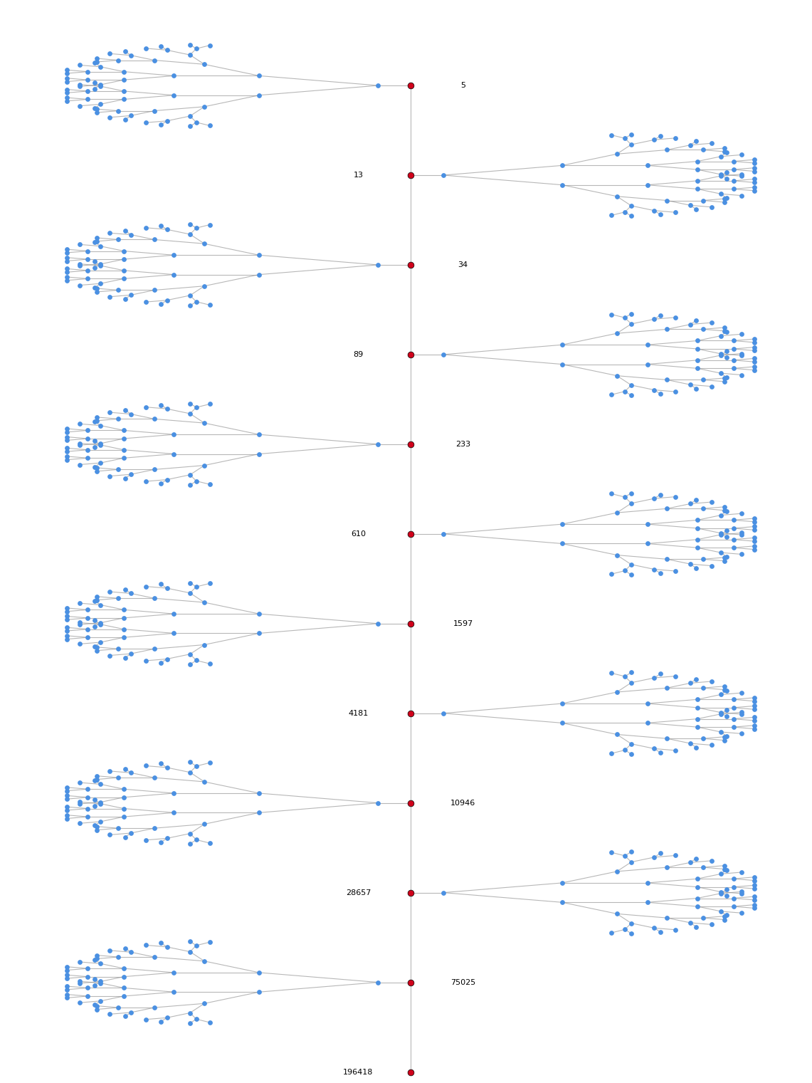
The Fibonacci spine (red) and the side branches (blue). Once you leave the spine, the magnitudes accelerate so fast that hitting a Fibonacci value starts to feel like a category error. For background on tree layouts, see the
Trees chapter of the Graph Drawing Handbook.
December 24, 2025
These slides by Michel Waldschmidt are an introduction to Markoff Numbers.
Selected References
- Baragar (1996), On the Unicity Conjecture
- Button (2001), Markoff Numbers & Continued Fractions
- Chen (2013), On the Frobenius Conjecture
- Zhang (2006), Proof of uniqueness for prime-power
- Tornero (2008), A Geometric Approach
- Lagisquet (2020), Markov tree / Stern–Brocot indexing
- Lee (2022), On the ordering of the Markov numbers
- Bowditch, Markoff triples and quasifuchsian groups
- Itsara et al. (2003), Combinatorial Interpretations
- Labbé (2022), The q-analog over words
December 23, 2025
I have been looking at the Open Problems for the 2025 Barbados Graph Theory Workshop.
This collection, compiled by Julien Codsi, features a number of intriguing problems.
December 19, 2025
Correction Width
Definition (Correction width with $k$ labels)
Let $G=(V,E)$ be a graph and let $k\ge 1$.
The correction width of $G$ with $k$ labels, denoted $\text{cw}_k(G)$,
is the minimum integer $d$ such that there exist:
- a linear ordering $\pi=(v_1,\dots,v_n)$ of $V$, and
- a partition of $V$ into $k$ (possibly empty) classes
\[ V = V_1 \,\dot{\cup}\, V_2 \,\dot{\cup}\, \cdots \,\dot{\cup}\, V_k, \]
satisfying the following local approximation property:
For each time step $t\in\{1,\dots,n\}$ let $V_{\lt t}:=\{v_1,\dots,v_{t-1}\}$
and let $N_{\lt t}(v_t):=N(v_t)\cap V_{\lt t}$ be the set of predecessors adjacent to $v_t$.
There must exist a template set $T_t$ of the form
\[
T_t \;=\; \bigcup_{i\in S_t}\bigl(V_{\lt t}\cap V_i\bigr)
\qquad\text{for some subset } S_t\subseteq [k]:=\{1,\dots,k\},
\]
such that
\[
\bigl|\,N_{\lt t}(v_t)\,\Delta\,T_t\,\bigr| \;\le\; d.
\]
Remark. For $k=2$ this yields exactly four possible templates
$\emptyset$, $V_{\lt t}$, $V_{\lt t}\cap V_1$, $V_{\lt t}\cap V_2$,
matching the "connect to none / all / group 1 / group 2" intuition.
Definition (Permutation-mutable error construction)
Fix integers $k\ge 1$ and $d\ge 0$.
A graph $G=(V,E)$ belongs to $\mathcal{G}^{\mathrm{perm}}_{\mathrm{error}}(k,d)$
if there exists a sequential construction of $G$ that proceeds in steps
$t=1,\dots,n$ adding vertices in some order $(v_1,\dots,v_n)$, together with:
- a label assignment $\ell_t(v_s)\in[k]$ for each already created vertex $v_s$,
- at each step $t$, an optional global relabeling by a permutation $\sigma_t\in S_k$ applied to all current labels (i.e., $\ell_{t}(x)=\sigma_t(\ell_{t-1}(x))$),
- a default connection mask $S_t\subseteq[k]$ specifying that, by default, the new vertex $v_t$ connects to every predecessor whose current label lies in $S_t$,
- and an error set $E_t\subseteq V_{\lt t}$ of size at most $d$, whose adjacencies to $v_t$ are toggled relative to the default rule.
Formally, after choosing $\sigma_t$, $S_t$ and $E_t$, the adjacency between $v_t$ and a predecessor $u\in V_{\lt t}$ is set to
\[
\mathbf{1}_{\{u v_t\in E\}}
\;=\;
\mathbf{1}_{\{\ell_t(u)\in S_t\}} \;\oplus\; \mathbf{1}_{\{u\in E_t\}},
\]
where $\oplus$ is XOR. The labels of the new vertex can be assigned arbitrarily in $[k]$.
Theorem (Equivalence)
For every graph $G$ and every $k\ge 1$,
\[
\text{cw}_k(G)
\;=\;
\min\bigl\{\, d\in\mathbb{N} \;:\; G\in \mathcal{G}^{\mathrm{perm}}_{\mathrm{error}}(k,d)\,\bigr\}.
\]
In particular, for $k=2$ this identifies $\text{cw}(G):=\text{cw}_2(G)$ with the minimum
per-step correction budget in the $2$-label permutation-mutable error model.
Proof.
(Forward direction.) Assume $\text{cw}_k(G)\le d$ as witnessed by an ordering
$\pi=(v_1,\dots,v_n)$ and a partition $V=\dot{\cup}_{i=1}^k V_i$.
Construct $G$ sequentially in this order.
Assign each vertex $v_t$ the fixed label $i$ with $v_t\in V_i$ and never relabel
(i.e., take all $\sigma_t=\mathrm{id}$).
At step $t$, let $T_t=\bigcup_{i\in S_t}(V_{\lt t}\cap V_i)$ be a template satisfying
$|N_{\lt t}(v_t)\Delta T_t|\le d$. Use the default connection mask $S_t$ (connect to all
predecessors with label in $S_t$), and set the error set to
$E_t := N_{\lt t}(v_t)\Delta T_t.$
Then $|E_t|\le d$ and, by construction, the toggling rule realizes exactly the desired
neighborhood $N_{\lt t}(v_t)$. Hence $G\in \mathcal{G}^{\mathrm{perm}}_{\mathrm{error}}(k,d)$.
(Reverse direction.) Assume $G\in \mathcal{G}^{\mathrm{perm}}_{\mathrm{error}}(k,d)$.
Fix a realizing construction in the order $(v_1,\dots,v_n)$.
Because each global relabeling is a permutation, labels are only renamed over time.
Define the final label of a vertex $x$ to be the label it has after the last step,
and let $V_i$ be the set of vertices of final label $i$. This yields a partition
$V=\dot{\cup}_{i=1}^k V_i$.
Now consider any step $t$ and any predecessor $u\in V_{\lt t}$.
Since relabelings are permutations, there exists a bijection $\rho_t:[k]\to[k]$ such that
the current label class $j$ at time $t$ corresponds exactly to the final class $\rho_t(j)$,
restricted to predecessors:
\[
\{u\in V_{\lt t}:\ell_t(u)=j\} \;=\; V_{\lt t}\cap V_{\rho_t(j)}.
\]
The default rule at step $t$ uses a mask $S_t\subseteq[k]$, hence the default neighborhood is
\[
T_t \;:=\; \{u\in V_{\lt t}:\ell_t(u)\in S_t\}
\;=\; \bigcup_{j\in S_t}\bigl(V_{\lt t}\cap V_{\rho_t(j)}\bigr),
\]
which is a union of predecessor-pieces of the fixed final partition.
The construction then toggles adjacency on at most $d$ vertices $E_t$, so
\[
N_{\lt t}(v_t) \;=\; T_t \,\Delta\, E_t
\qquad\Longrightarrow\qquad
|N_{\lt t}(v_t)\Delta T_t| \;=\; |E_t| \;\le\; d.
\]
Thus the same ordering and the final partition witness $\text{cw}_k(G)\le d$.
Combining both directions proves the claimed equality. $\square$
Remark (If merges are allowed).
If the mutable model permits non-bijective relabelings (merges), the reverse direction above
can fail: merging can temporarily collapse multiple classes and later recreate two labels,
allowing constructions with smaller $d$ than any fixed partition can support.
In that setting one should either restrict to permutations (as above) or define a
dynamic correction width where the partition is allowed to evolve.
December 17, 2025
The Shannon capacity of a graph $G$ is defined as $$\Theta(G) = \lim_{d \to \infty} (\alpha(G^d))^{1/d}.$$ The best lower bound for 7-cycle graph $C_7$ was obtained by finding an independent set of size 367 in the fifth power. This yields: $$\Theta(C_7) \geq \sqrt[5]{367} \approx 3.2578.$$ See arXiv:1808.07438 for details. Below is a Colab notebook generated with AlphaEvolve. It gives the same result.

Algorithm for Lower Bounding the Shannon Capacity of $C_7$
Problem Definition
The algorithm searches for the Maximum Independent Set (MIS) in the graph $G = C_7^n$, which is the strong product of $n$ copies of the 7-cycle.
- Vertex Set: $V = \mathbb{Z}_7^n = \{0, 1, \dots, 6\}^n$.
- Adjacency: Two vertices $u, v \in V$ are adjacent if and only if:
$$ \forall i \in \{1, \dots, n\}, \quad (u_i - v_i) \pmod 7 \in \{0, 1, 6\}. $$
(Note: $6 \equiv -1 \pmod 7$).
An independent set $S \subseteq V$ requires that for any distinct pair $u, v \in S$, they are non-adjacent. The size of this set establishes a lower bound for the Shannon capacity: $\Theta(C_7) \geq |S|^{1/n}$.
Methodology: Randomized Iterated Local Search
The approach implements a Ruin and Recreate strategy combined with greedy construction and local optimization.
- Initialization: The search is seeded either with a known structured subset (e.g., based on the pattern $\{0, 2, 4\}^n$) or a previous best solution.
- Greedy Construction: The algorithm maintains an array of "forbidden counts" for every vertex. It iteratively selects random valid vertices (count = 0) and updates the counts of their neighbors.
- Local Search (1-Swaps): Once the set is maximal, the algorithm attempts to escape local optima. It selects a vertex $u \in S$ and checks if it is "critical" (i.e., removing it liberates new vertices blocked only by $u$). If so, $u$ is removed, and the greedy process immediately fills the gap, effectively performing a $(1, k)$-swap optimization.
- Perturbation (Ruin and Recreate): If the solution size stagnates, the algorithm randomly removes approximately 10% of the vertices (Ruin) and refills the set using the Greedy Construction (Recreate).
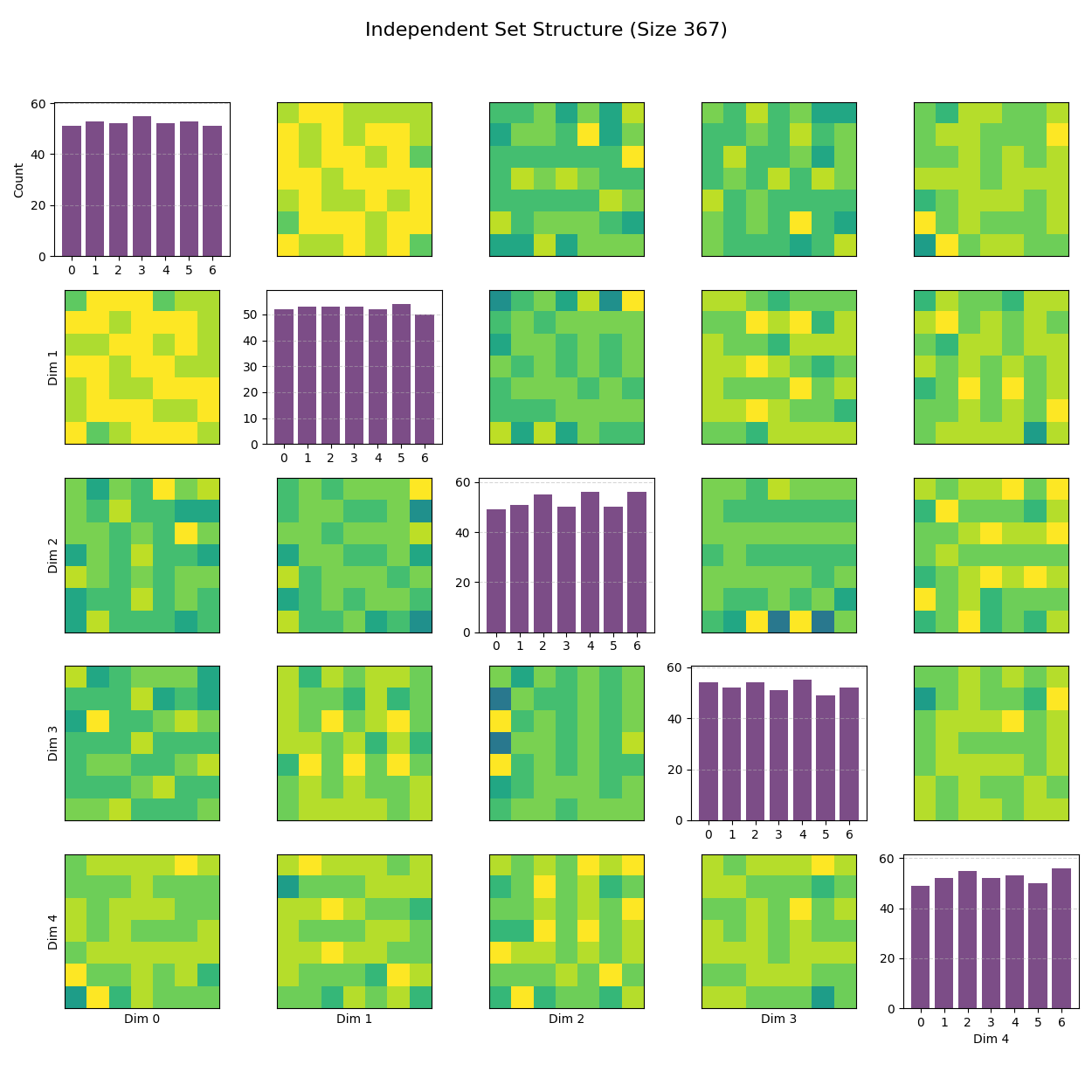
Structure of the Independent Set ($C_7^5$). The image is a $5 \times 5$ matrix of plots visualizing the structure of the Independent Set (IS) found in the 5-dimensional space ($C_7^5$). Here's how to read it:
Diagonal Plots (Top-Left to Bottom-Right): These are histograms for each of the 5 dimensions. They show the frequency of each coordinate value (0 through 6). For example, if you see taller bars at 0, 2, and 4, it means those values appear more frequently in that specific dimension, hinting that the solution might be built around a specific pattern like $\{0, 2, 4\}$.
Off-Diagonal Plots: These are 2D heatmaps showing the relationship between pairs of dimensions (e.g., Row 0, Column 1 shows Dimension 0 vs. Dimension 1). The color intensity (purple to yellow) represents the number of points at that specific $(x, y)$ coordinate pair. These projections reveal correlations. For an Independent Set in a strong product graph, you often see specific sparse patterns or "holes" because certain combinations of coordinates are forbidden to maintain the non-adjacency constraint.
Overall, this visualization helps verify if the solution is a structured product (e.g., looks like a clean grid) or a more random packing.